This technical brief on Lost Image Resolution has been provided by our valued supplier ITS.
You need 1080p video imagery? There are many parts needed to get there; expensive new lenses, cameras, storage and more. However, if you have compression such as H.264 or H.265 in the path, you’re not getting what you paid for!
Often HD recorders use compression to reduce video clip file size to fit on small storage (by today’s standards anyway). If your camera (source) and recorder, storage or displays (destination) are more than 500 feet apart, lost image resolution compression will likely be used to make it possible to transport the video.
As has been described in the TB series The Effects of Compression on Video Imagery, compression compromises many aspects of the source image; resolution is another degrading effect.
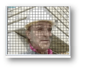
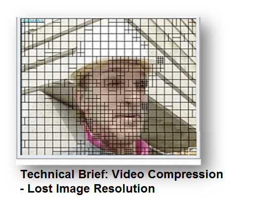
MPEG H.264 and H.265 compression encoders analyse each image in a video sequence to create reference and differential frames to meet the bit rate limits of the transport or storage capacity the system is connected to. All frames are essentially divided into a mosaic of different size blocks. The block sizes depend on the detail content of the image in each mosaic area. Reference frames are divided up into macroblocks like that shown in the construction foreman image. Each macroblock consists of an array of image samples (luma and chroma) as delivered by the camera using the sampling system in use (e.g. 4:2:2). Block sizes are 8×8, 16×16, 32×32. H.265 encoders can also merge adjoining macroblocks in large low detail areas. This tool contributes to the 50% compression efficiency of H.265. Exactly how each frame is divided into macroblocks, the criteria used by the encoder to determine block sizes and whether blocks can be merged are features of a particular encoder and are not controlled by any standard. This is in part why one can see image quality differences between encoders that meet H.264 and H.265 specification.
However the image is divided into macroblocks, each block is passed through a discrete cosine transform (DCT). The DCT essentially converts the spacial contours of the macroblock into an array of two-dimensional (2D) frequencies. An example of a standard array used by a decoder is shown at the left. The upper left corner represents “DC” that is a contourless area of some brightness. The lower right corner represents the highest frequency contour that can be represented in the array. The DCT provides a coefficient to use when applying each element of this array to reconstruct the original contour of the macroblock.
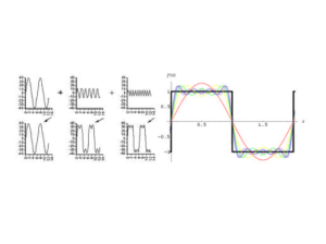
A zero value does not use the element. Coefficients can be any value; plus or minus and is an output of the DCT. This method in a single dimension is conceptually similar to how one transforms a time domain signal (waveform) to the frequency domain. Using the coefficients derived from a Fourier Transform of a square wave (both amplitude and phase) array of prototype sinusoids can be added together to reconstruct the time domain wave form as demonstrated in the figure to the right. Since the discrete transform is not a continuous spectrum there is a quantisation error built in to the reconstruction, however the size of the array (the one shown is 8×8 provides a 256 elements to use in reconstructing the luma contour of an 8×8 pixel array.
The colour samples (Cr and Cb) are processed the same way. Most cameras deliver 4:2:2 sampled imagery. The difficulty with that is the image sample is rectangular (two luma samples share one color sample) rather than square. In order to simplify the processing, most encoders wi ll convert the incoming 4:2:2 sampling to 4:2:0 sampling where 4 luma samples (brightness) share one colour sample. In doing so, there is some detail loss and colour shift. This can be observed when directly comparing the signals. Converting from 4:2:2 to 4:2:0 sampling effectively reduces the pixel bit depth from 20 bits to 15 bits. Digital image resolution is three dimensional, line count, pixels per line and bit depth. Although the number of pixels per line and line count are unchanged, the lower bit depth reduces fine image detail by limiting the dynamic range. That is, high contrast areas will suffer the most loss of detail. The encoder (compressor) is also tasked with managing the output bit rate to ensure that the video and data streams can be reliably transported to its ultimate destination. One tool is to manage the macroblock size. Areas of an image, such as sky, will not have much contour and therefore many coefficients of the DCT will be at or near zero. The larger you can make such areas, the more zero coefficients there are. Long runs of zero coefficients compress well without data loss (entropy encoding phase). The more zero coefficients the more entropy compression can be achieved.
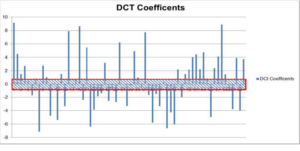
The illustration above models a histogram of coefficients of an image in an 8×8 macroblock array (64 elements).
Another tool available to the encoder is to adjust a value threshold where any DCT coefficients below an absolution magnitude of some value are set to zero. The strategy here is that decoding elements in the inverse DCT array that have small confidents will introduce small errors in the resulting macroblock reconstructed contour. As the available transport bit rate is restricted the encoder can increase the confident threshold thus creating more zero values and thereby increasing the entropy phase compression ratio. As can be seen some coefficients are very small.
The encoder can adjust the size of the threshold to eliminate elements of the array based on the value of the coefficient of the array. The elements are small contributors to reconstruction of the macroblock contour. Of course as this threshold is increased, so is the error between the source macroblock contour and the reconstructed contour.
The effect is similar to the frequency to time domain reconstruction of the square wave shown earlier. That is, if a frequency is dropped out of the sum, ripples appear in the top of the square and the rise and fall slopes deviate from the original input.
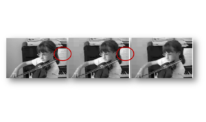
The contour is different from macroblock to macroblock, so the effect varies with the contour. In macroblocks having complex contours, the effective bandwidth of the sampling is often reduced (zero coefficients). Visually this can shift a fine detail to fuzzy in the macroblock. To what level the threshold is set however is determined by the overall bit rate required to deliver the video and data stream. Therefore the encoder will set the threshold based on what the aggregate bit rate of the stream of images after the DCT phase. In any particular macroblock the threshold may eliminate few if any array points; in others it may eliminate many. In the sequence of images below, the middle image is a reconstruction of the image at the far left. In this example take note of the sheet music in the background. In this case, the threshold eliminated enough high frequency components in the macroblock array to support the transport bit rate, that the music scale was obliterated (compare areas circled in red). This information is lost forever after the compression is complete.
As the macroblock size is increased, the complexity of the contour to recreate the sheet musing increases. However these elements create smaller DCT coefficients compared to the DC level and shading of the paper on which it is printed. The only way to prevent this information loss is to reduce the size of the macroblock at the target distance to reduce the complexity of the contour. This can be accomplished by reducing the size of the macroblock itself (32×32 to 16×16 or 8×8) or increasing the magnification. Increasing the magnification has the effect of reducing the target area a macroblock covers in the image.
An 8×8 array representing 64 raw video pixels is replaced by the threshold filtered DCT coefficients. The MPEG standards define how this information is communicated to a decoder. The decoder now only has the filtered data to perform and inverse DCT to recreate the pixel array contour. The decoded image is a mosaic of these recreated contours (macroblocks) sown together. In the TB Effects of compression on video imagery – Deblocking, it was shown how an algorithm can be applied to the decoded mosaic to hide the seams. This algorithm is not standardised and is often a differentiator for a decoder supplier relating to subjective image quality.
The image sequence of the girl with the violin above was used in the Deblocking article. Looking from left to right is the original image, the decoded image recreated from a mosaic of gradient macroblocks and at the far right, the same mosaic after deblocking where the edges of the mosaic elements are smudged out.
In addition to the lost detail regions around the macroblocks are smudged to hit the boundaries. This process further modifies the original image data. The modifications are permanent when captured as single images. The smudge itself may be different from decoder to decoder (supplier) cause fine detail differences from station to station, image capture to image capture.
How do you relate all of this to resolution loss? When the higher frequency elements of the inverse DCT array are removed edge details become fuzzy. The fuzziness can be thought of as progressively defocusing the lenses as high frequency elements are removed to meet bit rate limitations.
However what detail is compromised? Is it significant? The answer to that is a matter of scale. In a 1080×1920 image we can know the percentage of a 16×16 macroblock of pixels takes up on the image frame, but more important is what the complexity of the contour of the macroblock is. The complexity is determined in large part by what is in the image area of the macroblock at the target range.
As a way to exemplify the scale impact, two images were created to simulate macroblock area at the target where the lens zoom position would affect what detail is in the macroblock area. At the left represents an arbitrary lens setting. The image at the right represents looking at the same area with a narrower field of view (FOV). As you can see the complexity of the highlighted macroblock (red) in the left image is far greater than the complexity of the same macroblock where the FOV is smaller. In the left image, increases in threshold will wash out the details around the man’s eye. In the image to the right, the contour of the same macroblock is less complicated. It will produce fewer significant coefficients after the DCT is completed therefore preserving most of the detail during decode.
What is the resolution loss? The answer is complicated; it is image dependent, macroblock scale dependent and bit rate dependent. What detail is effected also depends on what is in the macroblock. Having said that, one can relate it to macroblock size, available bit rate and storage capacity. The lower the available bit rate, the smaller the macroblock area must represent at the target image to preserve the same or nearly the same detail delivered by the raw pixels at the source side.
Requiring more zoom and better optics to deliver an image with similar detail at the decoder side definitely translates to image resolution loss in the process. The resolution loss is not recoverable as the 2D elements created by the DCT at the encode side then zeroed to meet the bit rate limits are lost forever during the encoding process. Let us suppose a 1080p camera is being used to view and object 500 feet away. If a 1000 mm lens is used with a 25mm sensor the FOV would approximately be 1.5 degrees. The horizontal distance covered at the target range would be about 160 inches (13 feet). Each pixel at this range would cover 0.08 inches or approximately 0.007 inches2. The 8×8 macroblock covers about 0.43 inches2. What is the complexity of the image of a 0.007 inch2 are vs a 0.43 inch2 image area? Clearly the smaller the area covered by the macroblock the lower the detail loss.
Conversely, in order to compensate for compression encoder detail loss, the lower the bit rate, the greater the magnification needed. In specifying systems where compression is in the delivery path of the video, requirements must consider these effects.
The ITS 6520 Video Recording Instrument (VRI) captures uncompressed HD- SDI video. No color shift, quantization errors, no DCT coefficient losses; nothing missing, nothing lacking, nothing broken. You can play the clips just as the SDI from the camera delivered them. Playback in slow motion, single step frame to frame and loop on a subclip. Each frame presented is the full resolution and correct color just as the camera collected it. The actual video samples can also be downloaded via Ethernet to a file using our 6520 DownloadVideo© GUI. This ITS software product can also transcode the video to an uncompressed AVI clip, a compressed MP4 or Windows Media Video clip. Audio (if any) as well as imagery are captured, downloaded and transcoded. DownloadVideo© will also extract VANC metadata packets and with the key specification (see the KLV Software Toolkit for more information) can parse, format and display the data while playing the video with full frame synchronization. The DownloadVideo© Play function also permits one to search on data where video will play until the frame is found that meets the search criteria set.
If the devil is in the details, the details are important. Full resolution single frame shots are an integral part of analysis or evidence retention.
The 6520 Video Recording Instrument can be furnished with a removable 1Terabyte SSD. This capacity can hold a single 1080 clip of 151,500 frames. At 60 fps, 151K frames is 42 minutes of uncompressed 1080 video. However, it can hold 151K 1080 frames that may be comprised of many clips, up to 512 different clips can be captured to the SSD. The clips may even be different SD-SDI and HD-SDI formats.
For further information please contact us.